Edge principal components analysis example

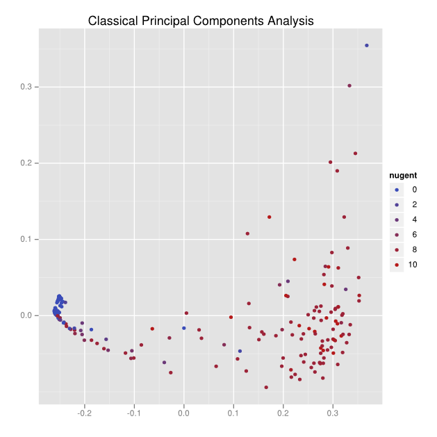
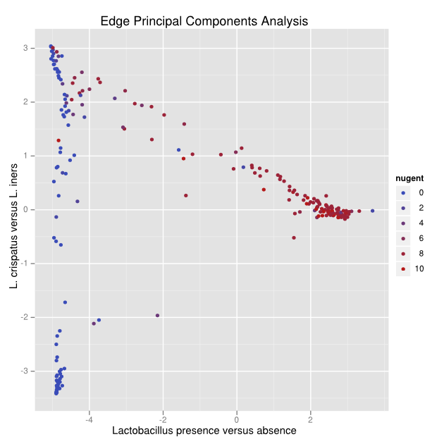
Here is a comparison of classical principal components analysis and edge principal components. As described in the paper, “nugent” is a clinical diagnostic score, where 0 represents a healthy vaginal microbiome, and 10 represents serious bacterial vaginosis. The plots are of 222 samples from a paper in preparation classified according to this score.

Classical principal components

Here’s the result of an application of classical principal components analysis to a distance matrix:

There can be no labeling for the axes, and the data is a small cluster on the left side and a big smear on the right.

Edge principal components

After an application of edge principal components, a pattern emerges.

To understand the pattern, we can look at the corresponding tree:

Reads placed on the red edges of the tree push points in the positive direction along that axis, while blue edges push in the negative direction. White edges make little or no difference. With this visual aid, we can see that the first principal component (click on the left hand tab labeled 0.6617974973) concerns Lactobacillus presence and absence, because all of the blue edges lead directly to the Lactobacillus clade. The second principal component (click on the right hand tab labeled 0.190879722165) is clearly comparing two different species of Lactobacillus, with those with L. crispatus reads pushing the sample points down and the L. iners pushing sample points up. The numbers in the tabs across the top are the fraction of variance “explained” by that principal component.

With that understanding we can interpret the pattern in the above figure: namely that there is a continuum from L. crispatus to L. iners, and from L. iners to low Lactobacillus, but not from L. crispatus to low Lactobacillus. The biological interpretation of this fact is reserved for our biology paper on this data set (under preparation).

For more details you can see a visual explanation (if your browser shows SVG) and our paper.