In late 2017 we were stuck without a clear way forward for our research on Bayesian phylogenetic inference methods.
We knew that we should be using gradient (i.e. multidimensional derivative) information to aid in finding the posterior, but couldn’t think of a way to find the right gradient. Indeed, we had recently finished our work on a variant of Hamiltonian Monte Carlo (HMC) that used the branch length gradient to guide exploration, along with a probabilistic means of hopping from one tree structure to another when a branch became zero. Although this project was a lot of fun and was an ICML paper, it wasn’t the big advance that we needed: these continuous branch length gradients weren’t contributing enough to the fundamental challenge of keeping the sampler in the good region of phylogenetic tree structures. But it was hard to even imagine a good solution to the central question: how can we take gradients in the discrete space of phylogenetic trees?
Meanwhile, in another line of research we were trying to separate out the process of exploring discrete tree structures with that of handling the continuous branch length parameters. As I described in a previous post, this combined a systematic search strategy modeled after what maximum-likelihood phylogenetic inference programs do, along with efficient marginal likelihood estimators to “integrate out” the branch lengths. This worked well for some data sets, but was bound to fail for any data set in which the posterior was spread across too many trees. Indeed, any method that needs to do a calculation on each tree in the credible set is bound to fail for large and flat posterior distributions.
At this point I was feeling despondent. I didn’t know how to take the gradient in discrete tree structure space, and the sampling-based methods we wanted to avoid seemed like the only approach that could work for flat posteriors. The only opportunity I could see was the Höhna-Drummond and Larget work on parametrizing tree structure posteriors, however we had previously shown that they were insufficiently flexible to represent the shape of true phylogenetic posteriors. Perhaps we could generalize them?
Cheng Zhang, when he was a postdoc in my group, took that vague idea and built a completely new means of inferring phylogenetic posteriors: variational Bayes phylogenetic inference. In this post I hope to explain this advance to the phylogenetics community.
How variational inference and the Metropolis-Hastings ratio each get around the normalizing constant problem
Bayesian phylogenetic inference targets the posterior distribution \(p(\mathbf{z} \mid D)\) on structures \(\mathbf{z}\) consisting of phylogenetic trees along with associated model parameters including branch lengths. Bayes’ rule tells us that the posterior is proportional to the likelihood times the prior:
\[p(\mathbf{z} \mid D) \propto p(D \mid \mathbf{z}) \, p(\mathbf{z})\]We can efficiently evaluate the two terms on the right hand side: the likelihood \(p(D \mid \mathbf{z})\) via Felsenstein’s tree-pruning algorithm and the prior \(p(\mathbf{z})\). However, it’s still quite hard to get correct values for the posterior \(p(\mathbf{z} \mid D)\) because of the unknown proportionality constant hidden in \(\propto\). We will call the likelihood times the prior on the right hand side of Bayes’ rule, \(p(D \mid \mathbf{z}) \, p(\mathbf{z})\), the unnormalized posterior.
The difficulty posed by the unknown proportionality constant is analogous to surveyors trying to calculate the average absolute height of a mountain range using only relative height measurements: they have to cover the entire mountain range before feeling confident that they can translate their relative measurements into an absolute estimate of the average height.
The Metropolis-Hastings algorithm avoids this problem by only working in terms of ratios of posterior probabilities. This cancels out the hidden proportionality constant, but with the cost of not directly giving an estimate of the posterior probability. Such an estimate then comes from running a Metropolis-Hastings sampler, which in the phylogenetic case doesn’t scale to data sets with many sequences as I described in a previous post.
Variational inference takes a different approach, fitting a variational approximation \(q_\phi(\mathbf{z})\) to the posterior \(p(\mathbf{z} \mid D)\). This approximation is parameterized in terms of some parameters \(\phi\). Once we have fit this approximation, we use it in place of our actual posterior for whatever downstream analyses we have in mind. It is an inferential method that can be used in place of Metropolis-Hastings.
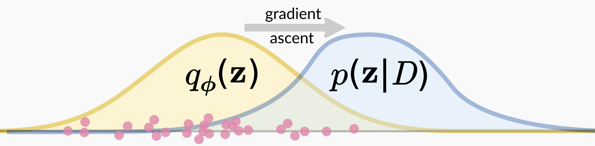
The fitting procedure for the variational approximation avoids the normalizing constant problem by taking a measure of “goodness of fit” that only requires evaluating the unnormalized posterior. In the most common formulation, this is the Kullback-Liebler divergence \(\text{KL}(q_\phi(\mathbf{z}) \parallel p(\mathbf{z} \mid D))\), in which the expectation of the normalizing constant \(\log p(D)\) can be pulled out. We can then ignore that constant when optimizing.
This optimization process happens by stochastic gradient descent, in which one samples from the current approximation \(q_\phi\) and uses that sample to take an optimization step in terms of \(\phi\) to improve the fit. That’s what I’m showing in the above figure, in which the pink points represent samples from the current variational approximation. We take those points and calculate a gradient in terms of the variational parameters \(\phi\) using the un-normalized posterior, and then take a gradient ascent step. I show a lot of points, corresponding to the fact that we use a multi-sample gradient estimator to decrease variance in the gradient estimate.
Intuitively, one can simply imagine that after a sample from \(q_\phi\) one would like to fiddle with \(\phi\) so as to improve fit of the variational approximation, just as if the posterior was “data” and we were fitting a statistical model. Early in the fitting procedure, this will involve increasing the probability of generating samples \(\mathbf{z}\) that had a high un-normalized posterior and decrease the probability of generating those that did not. If you want to learn more, see the excellent review article by Blei et al for background, and our ICLR paper for details about gradients.
However, I’d like to clarify a point that seems to cause confusion, including in the minds of reviewers who rejected our grant application: there is a clear distinction between the general technique of variational inference (VI) and a specific variational parameterization, such as mean-field VI. Mean-field VI makes strong independence assumptions which limits the flexibility of variational approximations; indeed it is not appropriate even for some simple hierarchical models. In contrast, VI is a general technique that will work given an appropriate approximating density and fitting algorithm. I describe evidence below that our parameterization for phylogenetic posteriors is sufficiently rich. More generally, there are now many methods that use more richer families of variational approximations such as normalizing flows.
How do we obtain a variational approximation of a phylogenetic posterior?
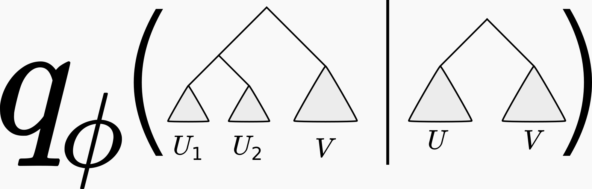
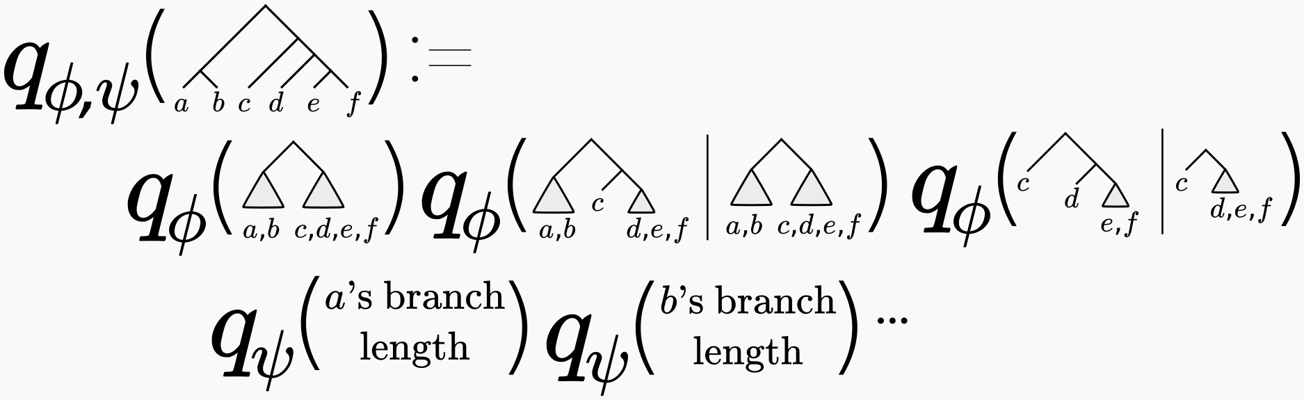
You may be thinking “well this all sounds very nice, but how are we going to parameterize a discrete set of phylogenetic trees using real-valued parameters \(\phi\)?” This is not at all obvious, and is the subject of a previous post (where we also credit to the originators of this approach). In short, one approximates the phylogenetic posterior using a series of conditional probabilities, like so:
We showed in our our 2018 NeurIPS paper that this parametrization was sufficiently rich to approximate the shape of phylogenetic posteriors on real data to high accuracy. In fact, in that paper (Table 1) we showed that the variational approximation fit to an MCMC sample was significantly more accurate than just using the MCMC samples in the usual way.
For full variational inference, we also layer on a variational distribution of branch lengths in terms of another set of variational parameters \(\psi\). I’m not going to describe how those work, but Cheng found a nice parameterization that used “just the right amount” of tree structure. See our 2018 ICLR paper for a full description.
With the complete variational parameterization in hand, all that remains is to fit it to the posterior. This required deft coding and a lot of tinkering on Cheng’s part, using control variate ideas for the tree structure and the reparametrization trick for branch lengths. The result? An algorithm that can outperform MCMC in terms of the number of likelihood computations.
The phylogenetic reader may also be interested in Table 1 of the ICLR paper, which shows that importance sampling using the full variational approximation gives marginal likelihood results quite concordant with, though with lower variance, than the stepping-stone method. Stepping-stone is a computationally expensive gold-standard method, whereas our method only required 1000 importance samples (and thus only 1000 likelihood evaluations once the variational approximation was fit). That’s promising!
What’s next?
We’re working hard to realize the promise of variational Bayes phylogenetic inference. On the coding front, we’re developing the libsbn library along with a team including Mathieu Fourment. The concept behind this Python-interface C++ library is that you can express interesting parts of your phylogenetic model in Python/TensorFlow/PyTorch/whatever and let an optimized library handle the tree structure and likelihood computations for you. It’s not quite useful yet, but we already have the essential data structures, as well as likelihood computation and branch length gradients using BEAGLE. I’m having a blast hacking on it, and it shouldn’t be too long before it can perform inference.
But the really fun part about variational inference is the ability to develop tricks that accelerate convergence. VI is fundamentally an optimization algorithm, and we can do whatever we want to do to accelerate that optimization. For example stochastic variational inference accelerates inference by taking random subsets of the data. We need to be careful about how to do that in the phylogenetic case (we can’t naively subsample tips of the tree) but we are currently pursuing ideas along those lines. In contrast, MCMC is a fairly constrained algorithm, and clever algorithms run the risk of either disturbing detailed balance or leading to an impossible-to-calculate proposal density.
I haven’t mentioned continuous model parameters other than branch lengths, and our initial work only used the simplest phylogenetic model: Jukes-Cantor without an explicit model of rates across sites. Mathieu is working out the gradients of nucleotide model parameters, which will allow us to formulate variational approximations of those too.
There’s still a lot to be done, and I’m having the time of my research life working in this area. I’d love to hear any comments, and don’t hesitate to reach out with questions.
We’re always interested in hearing from people interested in our work who might want to come work with us as students or postdocs. Please drop me a line!
I’m very grateful to Cheng Zhang for his creativity and skill in making this project happen. He is now now tenure-track faculty at Peking University in Beijing. I’d also like to thank our growing team of collaborators working on this subject.
Also, if you are interested in this area, check out the work of Mathieu Fourment and Aaron Darling, which is an independent development from ours.